A tutorial for solving Differential Equations in Julia
My research involves solving high ordered highly coupled differential equations. And while working in the last few years, I have used many programming languages like C, Fortran, Python, and Julia. I have also utilised softwares like Matlab and Mathematica for the same purpose thanks to the university wide license provided by my department.
I have realised that each had its own advantages. But among all of these, I found Julia to be the most superior among the computational capacity, variety, speed and ease of use. There already exist benchmarks published on the internet that looks at various ODE solvers or interfaces and rank them for their speed and efficiency. I will not be doing that in this post. This post is intended as a tutorial for those who wish to use Julia for solving differential equations. For more information on how Julia is the best at solving ODEs (ordinary differential equations), I will point you to benchmark link and resources at the end of the post.
Julia?
For people who are new to Julia, I will go through some introductory element and syntax in this post, which will be good for people starting with Julia, people who want to go into further details and want to spend more time learning it, see links at the end. For people who have used python which is common for science researchers, Julia looks very similar and is easy to grasp. I moved from python to julia myself and found a lot of common language rules and syntax. For people who want a tiny introduction to the syntax of Julia, you can jump below to the section where I introduce some concepts that are used in this post and would be beneficial.
DifferentialEquations.jl
We can write our own differential equations solver using the Euler or Runge Kutta methods, in pure Julia, but the developers have created a brilliant scientific library DifferentialEquations.jl which provides industry standard differential equations solver. In this post we will only be using this library exclusively for solving ODEs. You can install it using
julia>] add DifferentialEquationsOne dimensional ODE (Logistic Growth)
Let us take an example to learn how to use DifferentualEquations.jl, we will start with a one dimensional ODE.
Population growth with a carrying capacity (previously discussed in a blog post here.)
\[\frac{dN}{dt} =rN \cdot \left( 1- {\frac{N}{C}}\right) \]Here, \(N(t)\) is population at time \(t\), C is the carrying Capacity of the population, and \(r\) is the growth rate. This equation is famously known as the logistic growth dynamical equation and is important in various fields like physics, medicine, computers, networks, and ecology.
Let us use DifferentialEquations to solve this linear differential equation.
using DifferentialEquations
f_logistic(u,p,t)=p[1] * u * (1 - u/p[2])
u0 = 0.25
tspan = (0.0, 10.0)
params=[0.5,1.0]
prob = ODEProblem(f_logistic, u0, tspan,params)
sol = solve(prob, Tsit5(), reltol = 1e-8, abstol = 1e-8)
@show sol.u
sol.u = [0.22, 0.2214624947856733, 0.22839406288432468, 0.2397665944624233, 0.25353691189172606, 0.2718027963182323, 0.29429750259628623, 0.3233955825445172, 0.39217810003773756, 0.4254078760000628, 0.47122980934119635, 0.5110669792190305, 0.5536344555821728, 0.5942082113800929, 0.6347729254986635, 0.6741582191045536, 0.7131345538896132, 0.7524902118492397, 0.7993766630870759, 0.8272052545288429, 0.854428424597453, 0.875866364292772, 0.894764782343281, 0.9105737408909818, 0.9242005455844378, 0.9357992086733474, 0.9457537584482427, 0.9542691501119392, 0.9615658394979313, 0.9678068498963645, 0.9731399616235411, 0.9766682882615482]And voila, we have the solution. But wait? how did that work? Let us take it step by step.
We always solve the ODE system in two parts, we first define the problem: this involves defining (usually a function) the differential equations and then defining an ODEProblem object. The following line take care of the former:
f_logistic(u,p,t)=p[1] * u * (1 - u/p[2])Note the use of u is just arbitrary, I could just define it in terms of N and it would still give me the right result. p is an array of parameters defined for the function and given to ODEProblem as an input. The function has three inputs, first is the variable itself, second is an array p that includes all the parameters, and last is time t. This particular ODE was not explicitly time dependent. But we can have systems with explicit time dependence, so we always keep it in the skeleton.
tspan is a tuple which tells the system the timescale upto which the solution needs to be solved. So the solution \(N(t)\) will be from \(N(0)\) to \(N(10)\). And last but not the least u0 tells us the initial value, as in essence, the problem we are solving here is an initial value problem. Now, we get to the solution:
sol = solve(prob, Tsit5(), reltol = 1e-8, abstol = 1e-8)This line solves the problem defined using ODEProblem(f,u,t,p), the solve function takes the problem (prob here) as an input, the solver we are using to solve the ODE (Tsit5()) here is also mentioned, and the tolerance values upto which we will be solving.
abstol and reltol are different kind of tolerance values one can use for stopping the solver. They are absolute tolerance levels and relative tolerance levels. Absolute tolerance looks at successive values to check convergence, x{t+1}-x{t}<abstol, whereas the relative tolerance provides us with fractional convergence check.
The solver is a 5th order solver much like RK4-5. For people who have used matlab, it is equivalent to ode45 function there. Or for scipy users it is like the default solver of scipy's solve_ivp. Tsit5 uses a different parameter table than the usual RK45 method that gives better accuracy. See section below for more on the types of solvers available. There are dozens of solvers available..
This gives us an object sol, sol.u gives us \(N(t)\), whereas sol.t gives us an array with time values at which \(N(t)\) is evaluated. sol.t gives adaptive (non-uniform) time steps depending on the kind of solver.
The results we can then plot using any Plotting libraries in Julia. The most common is Plots.jl, the code to plot using Plots.jl is given below:
using Plots
function actual(r,C,n0,t)
    return C/(1+((C-n0)/n0)*exp(-r*t))
end
Plots.plot(sol, linewidth = 5, title = "Solution to the linear ODE and plotting with Plots.jl",xaxis = "Time (t)", yaxis = "N(t) (population)", label = "Numerical Solution (N(t))")
Plots.plot!(sol.t, t -> actual.(params[1],params[2],u0,t), lw = 3, ls = :dash, label = "Actual Solution")
Plots.savefig("ODE1d.png")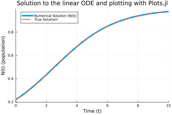
I prefer using CairoMakie.jl to do scientific plotting. It is more customisable and gives better quality plots (also as a personal choice, it looks better to me). Feel free to check out documentation for cairomakie linked at the bottom of the post.
using CairoMakie,LaTeXStrings
fig=CairoMakie.Figure()
ax=CairoMakie.Axis(fig[1,1],xlabel=L"\text{Time }(t)",ylabel=L"N(t)\text{ (population)}",title="Solution and plotting using Makie")
lines!(ax,sol.t,sol.u,label=L"\text{Numerical Solution }(N(t))",color=:black,linewidth=5)
lines!(ax,sol.t,t -> actual.(params[1],params[2],u0,t),label=L"\text{Actual Solution}",linestyle=:dash,color=:red,linewidth=3)
axislegend(position=:lt)
CairoMakie.save("Blog/2026/images/MakieODE.png",fig)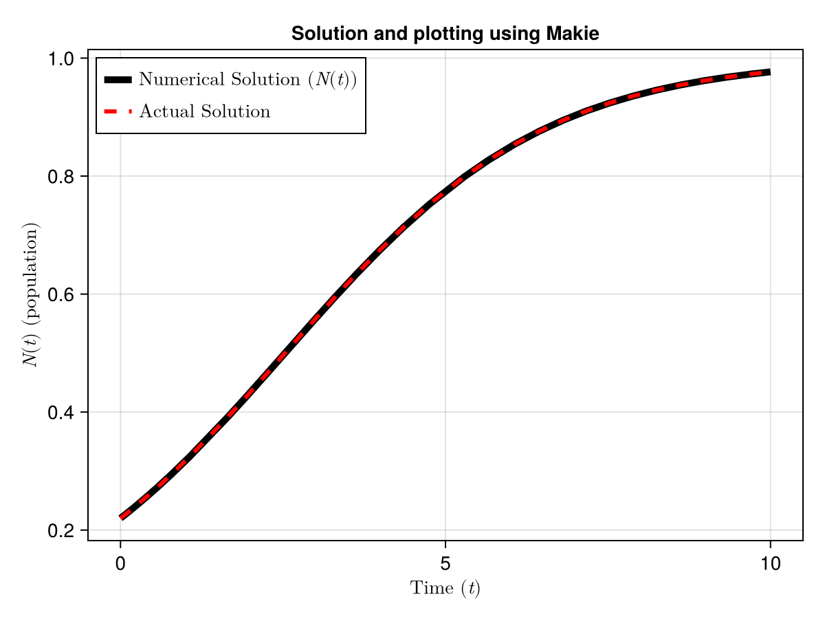
Higher dimensional ODE (Lorenz System, Chaos and strange attractor)
The most famous example for a higher dimensional ordinary differential equations system is the lorenz system. It has captured people's attention as the system that introduced the world to Chaos. We will try to solve the lorenz system using the Differential Equations julia library. The system is defined as:
\[ \begin{aligned} \frac{dx}{dt} &= a(y-x)\\ \frac{dy}{dt} &= x(b-z)-y\\ \frac{dz}{dt} &= xy-cz \end{aligned} \]Unlike the previous system, this one is non-linear and coupled. These equations actually represent fluid dynamics, where \(x\),\(y\) and \(z\) are different variables related to the rate of flow and the temperature profile of the fluid. It is not important what these physically mean for now. Parameters \(a\),\(b\) and \(c\) are important for studying different kinds of behaviours for the lorenz system.
We will take advantage of an important concept introduced in the section below. Mutable functions, or in-place updating functions, represented by the exclamation mark at the end of the name are used for better speed and memory efficiency. These functions updates the variables that are themselves inputs of the function. i.e. it updates already allocated variables. The compiler does not need to allocate the output of the function to another memory space and which in turn makes the solver much more efficient. The use of in-place updating functions get important when working with large \(N\) problems.
We can define the lorenz model in julia by
function lorenz_ODE!(du,u,p,t)
    du[1]=p[1]*(u[2]-u[1])
    du[2]=u[1]*(p[2]-u[3]) - u[2]
    du[3]=u[1]*u[2] - p[3]*u[3]
end
Note the extra du input to the function, this represents the du/dt values and it updates as the system solves for the solution. I can write it like this to make it more clear:
function lorenz_ODE!(du,u,p,t)
    dx,dy,dz=du[1],du[2],du[3]
    x,y,z=u[1],u[2],u[3]
    a,b,c=p[1],p[2],p[3]
    dx=a*(y-x)
    dy=x*(b-z)-y
    dz=x*y-c*z
end
It is better to write it in terms of arrays, instead of this with multiple variables for efficiency and it will be clear later why the former is better.
Now we can solve it just the way we did for the linear case. Defining the parameters:
params=[10.0,15.0,5.0]
tspan=(0.0,100.0)
u0=[1.0,0.0,0.0]
And the problem:
problem=ODEProblem(lorenz_ODE!,u0,tspan,params)ODEProblem with uType Vector{Float64} and tType Float64. In-place: true
Non-trivial mass matrix: false
timespan: (0.0, 10.0)
u0: 3-element Vector{Float64}:
1.0
0.0
0.0Finally the solution, just using the default solver:
sol=solve(problem)Okay, now we have the solution, let us plot it, I am going to use my trusty CairoMakie for plotting. You can use any library.
fig=CairoMakie.Figure()

ax1=CairoMakie.Axis(fig[1,1],xlabel="t",ylabel="x")
ax2=CairoMakie.Axis(fig[1,2],xlabel="t",ylabel="y")
ax3=CairoMakie.Axis(fig[2,1],xlabel="t",ylabel="z")
ax4=CairoMakie.Axis3(fig[2,2])

x=[sol.u[i][1] for i in 1:length(sol.u)]
y=[sol.u[i][2] for i in 1:length(sol.u)]
z=[sol.u[i][3] for i in 1:length(sol.u)]

CairoMakie.lines!(ax1,sol.t,x)
CairoMakie.lines!(ax2,sol.t,y)
CairoMakie.lines!(ax3,sol.t,z)
CairoMakie.lines!(ax4,x,y,z)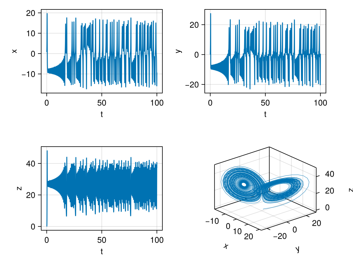
fig![Solution of the lorenz equations using DifferentialEquations.jl for parameters:[10.0,15.0,5.0]. The bottom right plot shows the `attractor` in the phase space. Other three plots are x,y and z with time.](/Blog/2026/images/lorenzspiral.png)
We can see for the parameters [10.0,15.0,5.0], we get a spiral attractor, i.e. all three values converge to a single point \((X,Y,Z)\).
We can change these parameters to get different results. With params=[10.0,28.0,8/3], we get the famous buttterfly wing shaped lorenz attractor, also known as the [strange attractor].
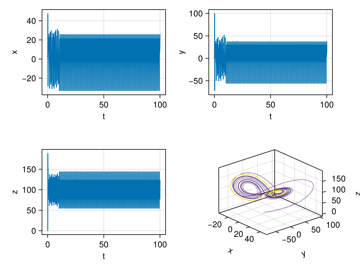
This chaotic strange attractor is present for a value of \(b\) beyond a critical value \(b_c\) for fixed \(a\) and \(c\) values. There are surprisingly a few interesting special values of \(b\) that shows periodic behaviour in the middle of chaos, for example, the following image is for params=[10.0,100.5,8/3]. The phase portrait is now colored by time, notice the late time convergence to a periodic attractor shown with yellow colored trajectory. This parameter value is originally from Chapter 4 of The Lorenz Equations by Colin Sparrow (1992, Springer) where he recognised multiple stable attractors.
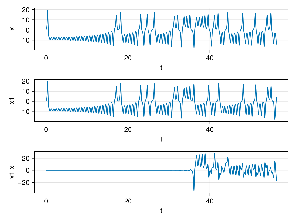
For fun, let us also show chaos, i.e. the sensitive dependence on initial conditions. I solve the ODEs for two intial conditions which are extremely close. u0=[1.0,0.0,0.0] and u01=[1.0,0.0,0.0+1e-9]. The starting position of z is just different by \(10^{-9}\). This slight difference leads to very different final result. We plot the \(x\) v/s \(t\) plot for both cases and also the difference between them.
Generalised Lotka Volterra Model (Ecological Predator-Prey Dynamics)
Alright, this is what we have been building upto, we are now going to be exploring a very high dimensional coupled ODE. Ecological systems like food webs can have hundreds of species interacting together and feeding in to each other. Solving such systems by explicitly writing the functions for each species could become, not impossible but a daunting task. What can we do?
We use a clever technique and take advantage of repeating functional forms for various species. Before defining the function though, let me talk about the generalised lotka volterra model, I have already talked about the prey predator dynamics and the lotka voltterra model in a previous post here, curious few can check it out. Let us dive straight in to the more generalised lotka volterra dynamics.
The GLV generalises ecological relationships between \(N\) species. The individual population \(x_i\) of \(i^{th}\) species evolves by the following set of ordinary differential equations:
\[ \frac{dx_{i}}{dt}=x_{i}\left(r_{i}+\sum _{j=1}^{n}A_{ij}x_{j}\right), \]Here, \(r_i\) are intrinsic growth rate of the species \(i\). It can be positive for birth , negative for death. This parameter combines both birth and death rate of the species. The value \(A_{ij}\) is the component of the interaction matrix, it gives us the effect of the species \(j\) has on to species \(i\). The diagonal terms, \(A_{ii}\) are taken to be negative, this provides a self-inhibition that stops exponential growth of individual population to infinity.
Okay, now that we know what the parameters are, let us solve the system, starting with defining the function. We are going to use all the tools that we have learnt together.
Note that we can distribute the equations in two parts:
\[ \frac{dx_{i}}{dt}=x_{i} \cdot f_i, \quad f_i=\left(r_{i}+\sum _{j=1}^{n}A_{ij}x_{j}\right) \]And \(\sum _{j=1}^{n}A_{ij}x_{j}\) is nothing but the \(i^{th}\) element of the product between \(A\) and \(\vec{X}\). So, we can take advantage of the LinearAlgebra.jl library and its in-place multiplication function mul!() to get Ax first. Then we can use the for loop to get dx[i].
````
Function to generate the generalised lotka volterra model
````
using LinearAlgebra
function GLV!(dx,x,par,t)
    ###############################################
    #par[1]=A_ij  par[2]=r(s)
    ###############################################
    Ax=zeros(eltype(x),length(x))  # creating a zero matrix of x datatype and with N=length(x) entries
    mul!(Ax,par[1],x) # Ax=A times X
    for i in 1:length(x)
        fi=par[2][i] + Ax[i]
        dx[i]=x[i]*(fi)
    end
end
Notice, how this generalizes for any \(N\), by using \(length(x)\) to determine \(N\). We can simplify this further by performing element wise operations that Julia allows.
````
Simpler function to generate the generalised lotka volterra model
````
using LinearAlgebra
function GLV_simple!(dx,x,par,t)
    ###############################################
    #par[1]=A_ij  par[2]=r(s)
    ###############################################
    Ax=zeros(eltype(x),length(x))
    mul!(Ax,par[1],x)
    fi=par[2] .+ Ax
    dx .= x.*(fi)
end
The for loop vanishes helping computational speed and making it very simple. We could infact write the last two lines in just one dx.= x.*(par[2] .+ Ax) for even better efficiency. But I choose to divide it for easier understanding.
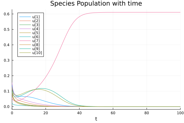
Case 1: Stable coexistence:
If we have weak inter-species interaction and strong self regulation, we usually end up with coexistnece. Here is a 3-species manufactured example. Off diagonal elements are considerably smaller than the diagonal elements. We keep intrinsic growth rates as constant.
N=3
A = [-1.0  -0.1  -0.05;
     -0.1  -1.0  -0.1;
     -0.05 -0.1  -1.0]
R = [1.0, 1.0, 1.0]
X0=Random.rand(N)
X0=X0./sum(X0)
params=[A,R]
prob=ODEProblem(GLV_simple!,X0,(0.0,100.0),params,reltol=1e-14)
sol=solve(prob,
        Tsit5(),
    save_everystep=true)
vec=abs.(sol.u[length(sol.u)])
println(vec)
Plots.plot(sol,title="Species Population with time",xlabel="t")
Plots.savefig("3species_coexist.png")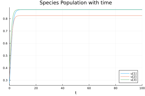
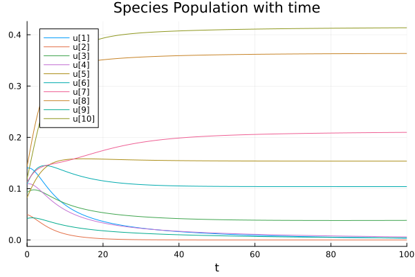
We can generalise it for a higher dimensional system making sure \(A_{ij}> |A_{ii}|\). In the following image, we sample the interaction elements from a normal distribution with mean 0.3 and standard deviation 0.1. Keeping diagonal elements at \(-1\) and also sampling \(r_i\) from a normal distribution around 0.5 with standard deviaiton 0.1 (Code below).
Case 2: Competitive Exclusion
Competitive exclusion is the idea in ecology which says that two species cannot coexist in one niche assuming resources are finite, either one or both species would eventually die.
We can model this behaviour by considering a toy model with
\[ A=\begin{pmatrix} -1.0 & -1.5 \\ -1.5 & -1.0 \end{pmatrix} \text{ and } R=[1,1] \]Solving this model, we notice it is dependent on the initial condition, if we start with more individuals of a species, we get that species taking over in the ecosystem.
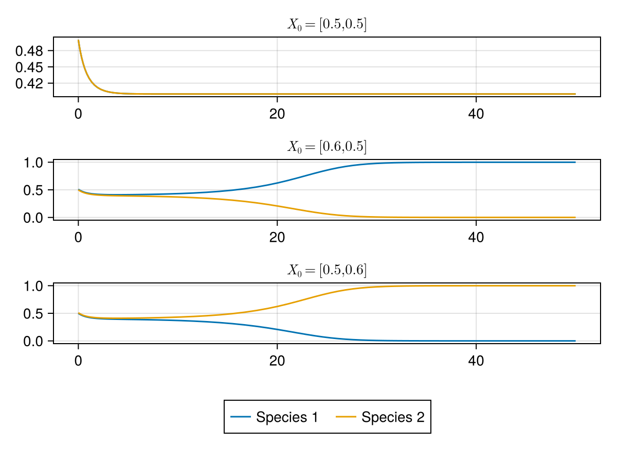
We can model it for higher species using our code, by considering the \(A_{ij}\) to be higher than the diagonal but of similar values. And higher than their own intrinsic growth rate. Here I sample the off diagonal elements from normal distribution with \(\mu =-1.3 , \sigma = 0.1\)
Case 3: Limit Cycle (oscillations)
If we take a pure predator-prey model, we usually see oscillatory patterns. A prey predator system have opposite signs in the symmetric values of the interaction matrix. \(A_{ij}=-A_{ji}\). We use small self regulation term to ensure species do not go extinct and can sustain oscilation. And we ensure predators have negative intrinsic growth rate because otherwise, preys would not be sufficient and it will not show cycles.
A = [-0.01   -1.0;
      0.5    -0.01]
R = [1.0, -1]  # predator has negative intrinsic growth
X0=[1/2,1/2]
params=[A,R]
prob=ODEProblem(GLV_simple!,X0,(0.0,50.0),params,reltol=1e-14)
sol=solve(prob,
        Tsit5(),
    save_everystep=true)
Plots.plot(
    Plots.plot(sol,title="Species Population with time",xlabel="t"),
    Plots.plot(sol,idxs=(1,2),title="Phase Portrait"))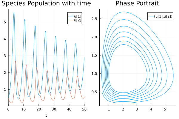
We can cleverly study oscillations and choatic behaviour in higher dimensional LV dynamics. But I will leave it for another day. This post is already too long. Note, that here we have allowed fractional values, in a more concrete simulation, if we are simulating population growth, we would work with discrete numbers and we would solve a stochastic differential equation instead. This is a more general look at the GLV.
Conclusion
I hope this blog post would help someone who is starting out with solving Ordinary Differential Equations using Julia. I understand the learning curve could be a little difficult at first to climb, but it is smooth scaling once you get a hang of it. We also looked at two very interesting dynamical systems and explored a few fun elements shown by the systems. Both individual systems can be explored a lot more thatn what has been done here.
Appendix
Short introduction to Julia's syntax
You can use Julia in its REPL, or download the IJulia package to use Julia in your jupyter notebook. Also see Pluto.jl for Julia's own unique notebook environment for more advanced users.
There are various datatypes much like python:
w=5
x=1.0
y=true
z=2 + 1im
typeof(w),typeof(x), typeof(y), typeof(z) # Diffenent Datatypes
(Int64, Float64, Bool, Complex{Int64})We can create for loops, while loops and perform all basic operations:
for x in [1,10,4,5]
    println("x=$x, x^2 = $(x^2), x+1=$(x+1), x/2=$(x/2)") #$ can be used to print variables in string, println adds a newline at the end
end
x=1, x^2 = 1, x+1=2, x/2=0.5
x=10, x^2 = 100, x+1=11, x/2=5.0
x=4, x^2 = 16, x+1=5, x/2=2.0
x=5, x^2 = 25, x+1=6, x/2=2.5
We can use arrays, and push elements into arrays. A fun thing that julia offers is using Latex symbols in code, for example the use of \(\in\) instead of in:
a=[]
for x ∈ 1:4
    push!(a,x)
end
@show a
println("You can also remove elements from the array")
pop!(a) # remove last element
@show a
popfirst!(a) # or remove first
@show a
a = Any[1, 2, 3, 4]
You can also remove elements from the array
a = Any[1, 2, 3]
a = Any[2, 3]
You can also use other latex symbols like \(\neq\), \(\notin\), \(\ge\), etc for computation.
a = [4, 5, 6]
b = Int8[4, 5, 6]
@show a
@show b
println("Arrays are typed — once defined, you cannot push an incompatible type:")
try
    push!(b, 2.5)   # Float64 into an Int8 array → error
catch e
    println("Caught error: ", e)
end
println("But this works fine:")
push!(b, Int8(7))
@show b
a = [4, 5, 6]
b = Int8[4, 5, 6]
Arrays are typed — once defined, you cannot push an incompatible type:
Caught error: InexactError(:Int8, Int8, 2.5)
But this works fine:
b = Int8[4, 5, 6, 7]
You can use inline for loop syntax for faster computation.
x=[1,2,3]
y=[var*4 for var in x]
@show y
y = [4, 8, 12]
A unique element of Julia is the use of element wise operations. Much like Python's numpy arrays, you can perform elementwise operations on Julia arrays, but the difference is that you can do that for any julia object and perform any functions elementwise.
x=range(1,10)
y=x.*2
@show y
z=[0.01,0.1,1,10,100,1000]
@show log10.(z)
y = 2:2:20
log10.(z) = [-2.0, -1.0, 0.0, 1.0, 2.0, 3.0]
Any function can be broadcast elementwise with ., this is more general than numpy. We have used this feature in the GLV_simple!() function in the post.
f(x, a) = exp(-a * x) * sin(x)
t = 0:0.1:10
@show y = f.(t, 0.3)   # broadcast over t, scalar a
y = f.(t, 0.3) = [0.0, 0.09688289328380166, 0.18709972965370564, 0.27008513274559637, 0.34538308622605984, 0.412645385178517, 0.4716290381244547, 0.5221927082502216, 0.5642922874073557, 0.5979757001718782, 0.6233770377206788, 0.640710122557378, 0.6502616052522163, 0.6523836934156877, 0.6474866111765241, 0.6360308845603287, 0.6185195444499075, 0.5954903343404111, 0.5675080049728184, 0.5351567722308355, 0.4990330085122907, 0.4597382312295467, 0.41787244524589484, 0.37402788900566825, 0.3287832269511704, 0.28269822362190966, 0.23630892767904832, 0.1901233870634137, 0.14461790964634494, 0.10023387713065636, 0.05737511365949082, 0.016405804642763814, -0.02235104424331126, -0.058614623052723865, -0.0921468283971277, -0.12275229312365146, -0.1502779625493469, -0.17461224813789056, -0.19568379217188714, -0.2134598791318406, -0.2279445311474595, -0.23917632605026343, -0.2472259772447618, -0.252193714849179, -0.2542065073598053, -0.2534151624927088, -0.24999134488260424, -0.2441245470031795, -0.2360190480499283, -0.2258908936306141, -0.213964926975803, -0.20047190004879267, -0.18564569043705717, -0.16972064728197822, -0.15292908678534597, -0.13549895505405088, -0.11765167324129497, -0.09960017714471167, -0.08154716065823255, -0.06368352977260994, -0.04618707120416317, -0.029221337225147054, -0.012934745892305753, 0.0025401063597654434, 0.017086924861838743, 0.030605996584895816, 0.043014278451087705, 0.05424530430318891, 0.06424892207637221, 0.07299087383860349, 0.080452232289178, 0.08662870803074772, 0.0915298424624241, 0.09517810148585773, 0.09760788537987573, 0.09886447019110424, 0.09900289581810379, 0.0980868156461157, 0.09618732213071121, 0.09338176214436016, 0.08975255520367502, 0.08538602690071788, 0.08037126898339726, 0.0747990365817965, 0.06876069207336287, 0.06234720403409254, 0.05564820864867913, 0.048751139863038584, 0.041740433470113664, 0.034696809236102924, 0.027696634110201256, 0.020811368526687513, 0.014107096812933094, 0.0076441417688952575, 0.001476762590162441, -0.004347065526096535, -0.00978579251958988, -0.01480435847344433, -0.01937418623529929, -0.02347310594634729, -0.027085216241410345]
using command. Or you can use import and as:
using LinearAlgebra

A=diagm([1,2,3,4]) # Diagonal matrix
@show A
@show eigen(A).values # eigenvalues

import Statistics as st

@show st.mean(A)
A = [1 0 0 0; 0 2 0 0; 0 0 3 0; 0 0 0 4]
(eigen(A)).values = [1.0, 2.0, 3.0, 4.0]
st.mean(A) = 0.625
Julia functions can return multiple values as a tuple natively — no need for a container:
function stats(x)
    return minimum(x), maximum(x), sum(x)/length(x)
end
lo, hi, avg = stats([3, 1, 4, 1, 5, 9])
@show lo, hi, avg
(lo, hi, avg) = (1, 9, 3.8333333333333335)
About solvers
DifferentialEquations.jl provides a large variety of solvers. The choice of solver significantly affects speed and accuracy. Here are the some of the common ones:
| Solver | Type | When to use |
|---|---|---|
Tsit5() | Explicit RK (5th order) | Default for non-stiff ODEs. As I said above, it is equivalent to ode45 in MATLAB |
RK4() | Explicit RK (4th order) | Simple fixed-step problems |
Vern7() / Vern9() | Explicit RK (7th/9th order) | High accuracy non-stiff problems |
Rodas5() | Implicit (stiff) | Stiff systems |
CVODE_BDF() | Implicit (stiff) | Very large stiff systems , import Sundials.jl package to use it |
lsoda() | Automatic stiffness switching | best when you do not know if the system is stiff or not or it changes in between. Import LSODA.jl to use |
KenCarp4() | IMEX | Mixed stiff/non-stiff (e.g. reaction-diffusion) |
A system is stiff when it contains dynamics at very different timescales simultaneously. Like fast-slow timescale problems. Explicit solvers like Tsit5 will take extremely small steps (very slow) on stiff systems. If your solver is slow or fails, try Rodas5().
You can also let the package choose automatically:
sol = solve(prob) # auto-selects solver based on problem typelsoda() is a julia wrapper for the classic Fortran LSODA solver. It is fast and robust for compisite problems.
Important links
DifferentialEquations.jl
DifferentialEquations.jl GitHub — Source and overview of the full SciML ecosystem
DifferentialEquations.jl Documentation — Official documentation, solver listings, and tutorials
SciML Solver Benchmarks — Benchmarks comparing Julia ODE solvers against MATLAB, Python (scipy), R, and Fortran implementations
Julia Learning Resources
Julia Official Documentation — Getting Started — The official first-stop for new Julia users
Julia Learning Page — Curated list of tutorials, courses, and community resources maintained by the Julia organisation
JuliaAcademy — Free video courses prepared by core Julia developers, including beginner and domain-specific tracks
Plotting
CairoMakie Documentation — CairoMakie backend reference, recommended for publication-quality static plots
Makie.jl Full Documentation — Complete Makie ecosystem docs covering CairoMakie, GLMakie, and WGLMakie
Julia Data Science — CairoMakie Chapter — Practical CairoMakie tutorial with worked examples
Previous posts referenced in this article
Code for plots
Competitive exclusion
Code for the figure for competitive exclusion for one species.
N=2
A = [-1.0  -1.5;
     -1.5  -1.0]
R = [1.0, 1.0]
X0=[1/2,1/2]
e=0.01
X01=[0.5+e,0.5]
X02=[0.5,0.5+e]
params=[A,R]
prob=ODEProblem(GLV_simple!,X0,(0.0,50.0),params,reltol=1e-14)
sol=solve(prob,
        Tsit5(),
    save_everystep=true)
prob1=ODEProblem(GLV_simple!,X01,(0.0,50.0),params,reltol=1e-14)
sol1=solve(prob1,
        Tsit5(),
    save_everystep=true)
prob2=ODEProblem(GLV_simple!,X02,(0.0,50.0),params,reltol=1e-14)
sol2=solve(prob2,
        Tsit5(),
    save_everystep=true)
fig=CairoMakie.Figure()
ax=CairoMakie.Axis(fig[1,1],title=L"X_0=[0.5,0.5]")
ax1=CairoMakie.Axis(fig[2,1],title=L"X_0=[0.6,0.5]")
ax2=CairoMakie.Axis(fig[3,1],title=L"X_0=[0.5,0.6]")
x=[sol.u[i][1] for i in 1:length(sol.u)]
x1=[sol1.u[i][1] for i in 1:length(sol1.u)]
x2=[sol2.u[i][1] for i in 1:length(sol2.u)]
y=[sol.u[i][2] for i in 1:length(sol.u)]
y1=[sol1.u[i][2] for i in 1:length(sol1.u)]
y2=[sol2.u[i][2] for i in 1:length(sol2.u)]
CairoMakie.lines!(ax,sol.t,x,label="Species 1")
CairoMakie.lines!(ax,sol.t,y,label="Species 2")
CairoMakie.lines!(ax1,sol1.t,x1)
CairoMakie.lines!(ax1,sol1.t,y1)
CairoMakie.lines!(ax2,sol2.t,x2)
CairoMakie.lines!(ax2,sol2.t,y2)
Legend(fig[4,1],ax,tellwidth=false,nbanks=2)
CairoMakie.save("Blog/2026/images/competitiveexclusion.png",fig)
Coeexistence
Code for coexistince of multiple species:
N=10
A=zeros(Float64,N,N)
for i in 1:N
    for j in 1:N
        if i==j
            A[i,j]=-1
        else
            A[i,j]= -0.3 + 0.1*randn() #2*Random.rand()-1#
        end
    end
end
X0=Random.rand(N)
X0=X0./sum(X0)
R=(1/2).+0.1.*Random.randn(N)
params=[A,R]
prob=ODEProblem(GLV_simple!,X0,(0.0,100.0),params,reltol=1e-14)
sol=solve(prob,
        Tsit5(),
    save_everystep=true)
Plots.plot(sol,xrange=(0,100))
Lorenz Sensitivity
fig=CairoMakie.Figure()
params=[10.0,28,8/3]
tspan=(0.0,100.0)
u0=[1.0,0.0,0.0]
u01=[1.0,0.0,0.0+1e-9]
problem=ODEProblem(lorenz_ODE!,u0,tspan,params)
sol=solve(problem,reltol=1e-10)
problem1=ODEProblem(lorenz_ODE!,u01,tspan,params)
sol1=solve(problem1,reltol=1e-10)
#ax4=CairoMakie.Axis3(fig[1,1],azimuth=1.275pi+pi/2)
ax1=CairoMakie.Axis(fig[1,1],xlabel="t",ylabel="x")
ax2=CairoMakie.Axis(fig[2,1],xlabel="t",ylabel="x1")
ax3=CairoMakie.Axis(fig[3,1],xlabel="t",ylabel="x1-x")
x=[sol.u[i][1] for i in 1:length(sol.u)]
y=[sol.u[i][2] for i in 1:length(sol.u)]
z=[sol.u[i][3] for i in 1:length(sol.u)]
x1=[sol1.u[i][1] for i in 1:length(sol1.u)]
y1=[sol1.u[i][2] for i in 1:length(sol1.u)]
z1=[sol1.u[i][3] for i in 1:length(sol1.u)]
#CairoMakie.lines!(ax4,x,y,z,linewidth=0.5,color=(:black,0.5))
#CairoMakie.lines!(ax4,x1,y1,z1,linewidth=0.5,color=(:red,0.5))
CairoMakie.lines!(ax1,sol.t[1:2000],x[1:2000])
CairoMakie.lines!(ax2,sol.t[1:2000],x1[1:2000])
CairoMakie.lines!(ax3,sol.t[1:2000],x[1:2000]-x1[1:2000])
fig
CairoMakie.save("Blog/2026/images/lorenzsensitivity.png",fig)
Lorenz Periodic
params=[10.0,100.5,8/3]
tspan=(0.0,100.0)
uo=[1.0,0.0,0.0]
problem=ODEProblem(lorenz_ODE!,u0,tspan,params)
sol=solve(problem,reltol=1e-10)
fig=CairoMakie.Figure()

ax1=CairoMakie.Axis(fig[1,1],xlabel="t",ylabel="x")
ax2=CairoMakie.Axis(fig[1,2],xlabel="t",ylabel="y")
ax3=CairoMakie.Axis(fig[2,1],xlabel="t",ylabel="z")
ax4=CairoMakie.Axis3(fig[2,2],azimuth=1.275pi+pi/2)

x=[sol.u[i][1] for i in 1:length(sol.u)]
y=[sol.u[i][2] for i in 1:length(sol.u)]
z=[sol.u[i][3] for i in 1:length(sol.u)]

CairoMakie.lines!(ax1,sol.t,x)
CairoMakie.lines!(ax2,sol.t,y)
CairoMakie.lines!(ax3,sol.t,z)
CairoMakie.lines!(ax4,x,y,z,linewidth=0.5,color=sol.t,colormap=:viridis)
fig
CairoMakie.save("Blog/2026/images/lorenzperiodic.png",fig)