Learn with me: Stochastic dynamics, fixed points and focker planck equations
I have studied non linear dynamics, both continuous and discrete systems in detail before. In my journey through the masters degree I encountered stochastic systems a lot but never sat down explicitly to learn actual stochastic systems and solving dynamical stochastic systems in detail. This post is supposed to be a self teaching guide I am writing up as I learn stochastic dynamics. In no manner should this post be considered a good introductory session to the models and solving non linear stochastic differential equations, I am sure both you and me can find better textbooks that will do a much better job at it.
Recently, I was trying to write a mean field version of a stochastic dynamical system and in the process of writing some discrete map which were probabilistic in nature, I realised I do not know what it means to have a stable fixed point in a stochastic system. I had a rough idea what it would imply. But I decided I think it will be worth it to just go through a small crash course. So, let us embark on this journey and learn some basics of stochastic dynamics.
From determinism to stochasticity
Classical dynamical systems rely on deterministic ordinary differential equations. Recently I had written a blog post for solving ordinary differential equations, all the systems we explored in that post were classical dynamical systems where the evolution of the system was dependent on either an ODE \(\dot{x} =f(x)\) or a deterministic map like \(x_{n+1}= f(x_n)\). In these systems, the long term behaviour is determined by the fixed points \(x^*\) where \(f(x^*)=0\). They are called fixed point because once they reach that point, they stay there, since the flow is zero.
What would happen if our differential equation has a noise term. In the sense that there are fluctuations that does not allow the system stay at the exact fixed point. Now, we know that if the fixed point is stable, if we perturb it the system will move back to the fixed point. Sometimes the story is not that straight forward.
Real-world systems, are constantly subjected to microscopic fluctuations, environmental uncertainty, and unknown forces collectively termed noise. In stochastic dynamical systems, noise fundamentally alters the topological landscape:
Static fixed points dissolve into probability distributions \(P(x)\), representing the relative likelihood of finding the system in a given state over time. We expect that \(P(x)\) will be peaked around the deterministic fixed point.
Point attractors become random attractors, defining statistically stationary wandering regimes rather than static convergence.
Discrete stochastic map
Let us consider the most simple example for a stochastic discrete system. This is a simple 1-D linear stochastic map defined by the following difference equation:
\[x_{n+1} = a x_n + \eta_n\]where \(a\) is a constant parameter (\(\vert{}a\vert{} < 1\) for linear stability) and \(\eta_n\) is independent and identically distributed (i.i.d.) Gaussian white noise with mean zero and variance \(\text{Var}(\eta) = \sigma^2\).
This noise is a standard noise used in mathematical modeling. We can take other noise functions, but for this post I will consider this as our noise function.
If there was no noise, the system would have a stable fixed point at \(x^*=0\), as \(a<1\). But with the noise, there will be a cloud with its own variation that we can calculate.
To find the stationary variance \(\text{Var}(x)\) of this process, we take the variance of both sides at steady state:
\[\text{Var}(x_{n+1}) = \text{Var}(a x_n + \eta_n)\] \[\text{Var}(x) = a^2 \text{Var}(x) + \sigma^2\]Solving algebraically for \(\text{Var}(x)\):
\[\text{Var}(x)(1 - a^2) = \sigma^2 \implies \text{Var}(x) = \frac{\sigma^2}{1 - a^2}\]Interpretation: When \(a\) approaches \(1\) , the denominator shrinks, causing the variance to explode.
We can simulate this stochastic map using Julia to visualise the time series.
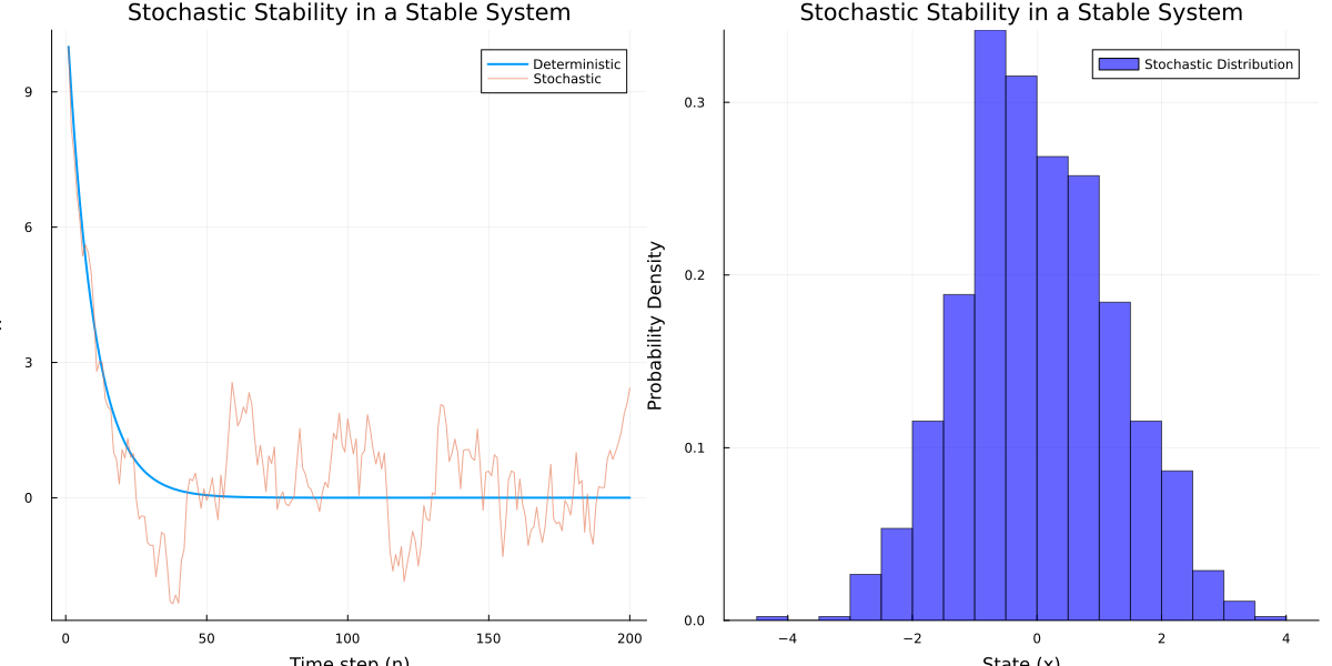
We note that the stochastic time series move to the deterministic fixed point and fluctuates around it with the variance dependent on \(\sigma\) and \(a\).
The size of the probability cloud is a balance between the noise (\(\sigma^2\)) and the deterministic stability (\(a\)). If \(a\) is close to 0 (very stable), the system tightly clusters near 0. If \(a\) approaches 1 (barely stable), the denominator shrinks and the variance explodes. The code is available at the end for those who wish to visualise this themselves.
Moving to two dimensions
In higher dimensional systems, we can have slow and fast modes depending on the spectral properties of the dynamical system. I will not be going into detail what it means and what the jacobian and its modes are defined as. But I will be now trying to understand what happens when there is stochastic noise in a 2d system.
Imagine a 2D system where we have linearized around a fixed point. For simplicity, let's assume the system is decoupled so the \(x\) and \(y\) axes act like two independent 1D maps, but with different eigenvalues (stabilities):
x-axis : \(x_{n+1} = \lambda_1 x_n + \eta_{x,n}\), where \(\lambda_1 = 0.1\)
y-axis : \(y_{n+1} = \lambda_2 y_n + \eta_{y,n}\), where \(\lambda_2 = 0.95\)
The slow mode, \(y\)-axis will have much larger variance while the fast mode, \(x\)-axis will quickly converge towards \((0,0)\). This means the noise accumulates heavily along the y-axis before the system can pull it back to zero.
We can visualise the stationary distribution for this 2D map by plotting scatter. Note, the variance along different axis and how they scale. We used same \(\sigma\) for each independent noise.
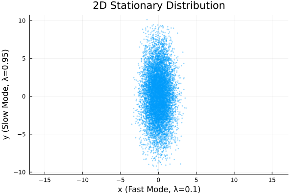
In our simple example, the two modes are independent of each other as there were no coupling terms between \(x\) and \(y\), but we can have more complex dynamics. In that case we do linearisations and calculate the eigenvector corresponding to the largest eigenvalue.
This is exactly why we use linearization around fixed points in nonlinear stochastic systems. We find the deterministic fixed point, compute the Jacobian matrix there, and those local eigenvectors tell us exactly how the noise will tilt and stretch the stationary distribution in that specific region. And from that we can visualise and plot \(P(x,y)\).
Stochastic Lyapunov Exponents
The Lyapunov exponent \(\lambda\) measures the average exponential rate of divergence (or convergence) of nearby trajectories, serving as the definitive test for stability and chaos:
\[\lambda = \lim_{t \to \infty} \frac{1}{t} \ln \left| \frac{\delta x(t)}{\delta x(0)} \right|\]To understand this in detail, let us derive very simple yet interesting results about this exponent.
We define the distance between two trajectories as \(d_n = x_n - y_n\).
For a nonlinear random map: \(x_{n+1} = f(x_n) + \eta_n\). If our two trajectories are infinitesimally close, the noise cancels out, and we can use a Taylor expansion (linearization) to see how the distance evolves:\(d_{n+1} \approx f'(x_n) \cdot d_n\) To find the overall stability, we calculate the Lyapunov exponent (\(\lambda\)), which is the long-term average of the exponential growth or decay rate of that distance:
\(\lambda = \lim_{N \to \infty} \frac{1}{N} \sum_{n=1}^N \ln \vert{}f'(x_n)\vert{}\)If we know the mathematical shape of that probability cloud—let's call its probability density function \(P(x)\), how could we use \(P(x)\) to calculate the Lyapunov exponent \(\lambda\) without having to run a massive time series simulation?
We simply calculate the expectation value of the lyapunov function:
\[\lambda = \int_{-\infty}^{\infty} \ln\vert{}f'(x)\vert{} \cdot P(x) \, dx\]Logistic Map, lyapunov constant and chaos
Logistic map is a famous discrete dynamical system which is simple in its form but shows incredibly complex behaviour ranging from stable fixed points, to period doubling and chaos.
The deterministic map is \(f(x) = r x (1 - x)\).
And our stochastic map is \(x_{n+1} = r x_n (1 - x_n) + \eta_n\)
The integral for the stochastic Lyapunov exponent of the Logistic Map becomes:
\[\lambda = \int_0^1 \ln\vert{}r(1-2x)\vert{} \cdot P(x) \, dx\]We first evaluate \(P(x)\) for the stochastic logistic map.
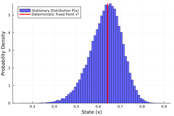
Once, we have \(P(x)\), we can evaluate the lyapunov integral.
x_star = 1 - 1/r  # Analytical fixed point
lyap_det = log(abs(r * (1 - 2 * x_star)))
#We approximate the integral over P(x) using the time-average of the trajectory
lyap_stoch = mean(log.(abs.(r .* (1 .- 2 .* x_stoch[1000:end]))))
Output:
Deterministic Fixed Point: x* = 0.6429
Deterministic Lyapunov Exponent: -0.2231
Stochastic Lyapunov Exponent: -0.4602
The negative \(\lambda\) tells us that for both deterministic and stochastic systems, the fixed point is stable.
If we consider \(r=4\), the logistic map is known to be chaotic. The lyapunov exponent is calculated as 0.6965. The positive value tells us that close curves diverge exponentially with postive exponent and thus they are choatic.
The Fokker-Planck Equation & Potential Landscapes
For continuous systems governed by a Stochastic Differential Equation (SDE):
\[\dot{x} = f(x) + \sigma \xi(t)\]where \(\xi(t)\) is Gaussian white noise, the evolution of the probability density function \(P(x,t)\) is governed by the Fokker-Planck Equation (forward Kolmogorov equation):
\[\frac{\partial P(x,t)}{\partial t} = -\frac{\partial}{\partial x} \big[ f(x) P(x) \big] + \frac{\sigma^2}{2} \frac{\partial^2}{\partial x^2} \big[ P(x) \big]\]To understand the origin of this equation, we can start by understanding a stochastic dynamical system in general. Let us say, we have a particle moving through space. We solve \(dx/dt\) to get the position of the particle and get its trajectory. Focker-Planck equation tracks how the entire cloud of probability distribution \(P(x,t)\) evolves over time.
At any moment, there are typically two forces that are evolving a stochastic dynamical system.
Drift: The deterministic part of the system, \(f(x)\), acts like a fluid current, sweeping the probability mass toward the stable fixed points.
Diffusion: The random noise acts like a stirrer, constantly spreading the probability mass outward, depending on the type of noise.
We can write the effect of the first process by deriving the expectation value of the fitness \(f(x)\), i.e. \(\frac{d}{dx}\left[ f(x)P(x) \right]\).
We write the effect of diffision as a flux: \(\frac{\sigma^2}{2} \frac{d^2}{dx^2} \big[ P(x) \big]\).
Deriving the Stationary Distribution
At steady state, the probability distribution ceases to evolve (\(\frac{\partial P}{\partial t} = 0\)), meaning drift flux and diffusion flux balance out:
\[0 = -\frac{d}{dx} \left[ f(x) P(x) \right] + \frac{\sigma^2}{2} \frac{d^2}{dx^2} P(x)\]Integrating once with respect to \(x\) :
\[f(x) P(x) = \frac{\sigma^2}{2} \frac{d}{dx} P(x)\]Rearranging terms:
\[\frac{P'(x)}{P(x)} = \frac{2f(x)}{\sigma^2} \implies \frac{d}{dx} \ln P(x) = \frac{2f(x)}{\sigma^2}\]Integrating both sides with respect to \(x\):
\[\ln P(x) = \frac{2}{\sigma^2} \int f(x) \, dx + C\]Exponentiating both sides introduces a normalization constant \(N = e^C\):
\[P(x) = N \exp\left( \frac{2}{\sigma^2} \int f(x) \, dx \right)\]The Potential Function
We define the potential function \(U(x)\) such that the deterministic drift is the negative gradient of the potential (\(f(x) = -U'(x)\) or \(U(x) = -\int f(x) \, dx\)):
\[P(x) = N \exp\left( -\frac{2 U(x)}{\sigma^2} \right)\]Analogy: This is mathematically identical to the Boltzmann distribution in statistical mechanics. The system acts like a particle rolling through a potential landscape \(U(x)\) while being thermally agitated by noise \(\sigma^2\).
An example can be \(f(x) = -kx\), what is the potential function \(U(x)\)? The potential becomes the simple harmonic potential and the probability distribution becomes the neat gaussian distribution:
\[ P(x)= N e^{-\frac{k x^2}{\sigma^2}}\]If we compare our result \(P(x) = N e^{-\frac{k x^2}{\sigma^2}}\) to the standard Gaussian formula \(e^{-\frac{x^2}{2\text{Var}(x)}}\), we can see that the variance of this continuous cloud is \(\text{Var}(x) = \frac{\sigma^2}{2k}\).
Just like the formula we derived for the discrete map (\(\frac{\sigma^2}{1-a^2}\)), the size of this continuous probability cloud is a direct ratio of the noise (\(\sigma^2\)) fighting against the deterministic stability (\(k\)).
Stochastic Bifurcations (P-Bifurcations)
Stochastic Bifurcations (P-Bifurcations)
A Phenomenological Bifurcation (P-bifurcation) occurs when a parameter variation triggers a qualitative change in the stationary probability distribution \(P(x)\) .
The Supercritical Pitchfork Potential
Consider the deterministic normal form for the pitchfork bifurcation.:
\[f(x) = r x - x^3\]Integrating to find the potential \(U(x) = -\int (rx - x^3)dx\):
\[U(x) = -\frac{r}{2}x^2 + \frac{1}{4}x^4\]When \(r < 0\): The potential features a single minimum at \(x = 0\). The distribution \(P(x) = N \exp(-\frac{2U(x)}{\sigma^2})\) exhibits a single central peak centered around the origin.
When \(r > 0\): The origin becomes a local maximum (unstable hill), and two symmetric minima emerge at the stable fixed points:
Because of the negative sign in the exponent of \(P(x)\), the potential's "W" shape is inverted into probability density: the two deep potential wells become twin probability peaks at \(x = \pm\sqrt{r}\), separated by a trough of low probability at \(x = 0\).
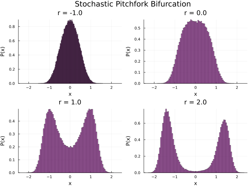
Note: We use a method known as Euler Maruyama method to numerically integrate the focker planck equation.
x[i+1] = x[i] + drift * dt + diffusion
Climate Application: Stochastic Resonance & the Benzi Model (1981)
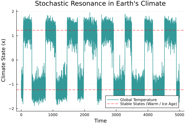
To explain how Earth transitions between glacial ice ages and warm interglacial periods despite weak orbital variations, Benzi et al. introduced a stochastic double-well model driven by periodic forcing link to main paper, we adapt that model into a simpler version:
\[\dot{x} = rx - x^3 + A\sin(\omega t) + \eta(\sigma)\]\(x\): Global temperature.
\(rx - x^3\): Climate feedback inspired from the double well potential
\(A\sin(\omega t)\): Weak periodic orbital variation (astronomical wobble of the earth).
\(\eta(\sigma)=\sigma \xi(t)\): Short-term stochastic weather fluctuations.
The idea behind this is to match the period of oscilations \(2\pi/\omega\) to the time of escape from the double well potential. The feedback between \(sin(\omega t)\) and double well forcing ensures that the potential landscape wobbles between one minima to other. Just as the barrier reaches its minimum, stochastic weather noise provides the necessary energy kick to push the system across the barrier to the other minima.
Code
Figure 1
using Random, Statistics, Plots

function simulate_maps(a, sigma, steps)
    x_det = zeros(steps)
    x_stoch = zeros(steps)

    # Start both far from the origin
    x_det[1] = 10.0
    x_stoch[1] = 10.0

    for n in 1:(steps-1)
        # Deterministic: strict fixed point
        x_det[n+1] = a * x_det[n]

        # Stochastic: kicked by random noise
        x_stoch[n+1] = a * x_stoch[n] + sigma * randn()
    end

    return x_det, x_stoch
end

# Set parameters for a stable system
a = 0.99
sigma = 0.5
steps = 1000

x_det, x_stoch = simulate_maps(a, sigma, steps)

# Visualizing the time series
p=plot(x_det[1:500], label="Deterministic", linewidth=2, xlabel="Time step (n)", ylabel="x")
plot!(p,x_stoch[1:500], label="Stochastic", alpha=0.6)

p1=histogram(x_stoch[100:end], normalize=:pdf, bins=30,
          label="Stochastic Distribution",
          xlabel="State (x)", ylabel="Probability Density",
          alpha=0.6, color=:blue, legend=:topright)
p=plot(p, p1, layout=(1,2), size=(1200,600), title="Stochastic Stability in a Stable System")
Figure 2
using Random, Plots

function simulate_2d_stochastic(lambda_x, lambda_y, sigma, steps)
    x = zeros(steps)
    y = zeros(steps)

    # Start at the origin
    x[1] = 0.0
    y[1] = 0.0

    for n in 1:(steps-1)
        # Fast mode
        x[n+1] = lambda_x * x[n] + sigma * randn()
        # Slow mode
        y[n+1] = lambda_y * y[n] + sigma * randn()
    end

    return x, y
end

# Parameters
lambda_1 = 0.1   # Fast mode (tightly bound)
lambda_2 = 0.95  # Slow mode (loose, high variance)
sigma = 1.0
steps = 10000    # More steps give a better picture of the distribution

x_vals, y_vals = simulate_2d_stochastic(lambda_1, lambda_2, sigma, steps)

# Visualizing the cloud
scatter(x_vals, y_vals,
        title="2D Stationary Distribution",
        xlabel="x (Fast Mode, λ=0.1)",
        ylabel="y (Slow Mode, λ=0.95)",
        legend=false,
        markersize=1.5,
        markerstrokewidth=0,
        alpha=0.4,
        aspect_ratio=:equal) # Equal aspect ratio shows the true stretching
Figure 3
using Random, Statistics, Plots

function simulate_logistic(r, sigma, steps)
    x_det = zeros(steps)
    x_stoch = zeros(steps)

    x_det[1] = 0.5
    x_stoch[1] = 0.5

    for n in 1:(steps-1)
        # Deterministic map
        x_det[n+1] = r * x_det[n] * (1 - x_det[n])

        # Stochastic map (clamped to keep the state within the [0,1] domain)
        noise = sigma * randn()
        x_stoch[n+1] = clamp(r * x_stoch[n] * (1 - x_stoch[n]) + noise, 0.001, 0.999)
    end

    return x_det, x_stoch
end

# Set parameters
r = 2.8       # Stable regime for the deterministic map
sigma = 0.05  # Noise intensity
steps = 50000

x_det, x_stoch = simulate_logistic(r, sigma, steps)

# --- 1. Deterministic Fixed Point and Stability ---
x_star = 1 - 1/r  # Analytical fixed point
lyap_det = log(abs(r * (1 - 2 * x_star)))

# --- 2. Stochastic Stability ---
# We approximate the integral over P(x) using the time-average of the trajectory
lyap_stoch = mean(log.(abs.(r .* (1 .- 2 .* x_stoch[1000:end]))))

println("Deterministic Fixed Point: x* = ", round(x_star, digits=4))
println("Deterministic Lyapunov Exponent: ", round(lyap_det, digits=4))
println("Stochastic Lyapunov Exponent: ", round(lyap_stoch, digits=4))

# --- 3. Visualizing P(x) ---
histogram(x_stoch, normalize=:pdf, bins=100,
          label="Stationary Distribution P(x)",
          xlabel="State (x)", ylabel="Probability Density",
          alpha=0.6, color=:blue, legend=:topleft)
vline!([x_star], label="Deterministic Fixed Point x*", color=:red, linewidth=3)
Figure 4
using Random, Plots

function simulate_climate(r, A, omega, sigma, dt, steps)
    x = zeros(steps)
    x[1] = -sqrt(r) # Start in the cold glacial state (left well)

    for i in 1:(steps-1)
        t = i * dt
        # Deterministic drift + weak orbital wave
        drift = r * x[i] - x[i]^3 + A * sin(omega * t)

        # Stochastic diffusion (weather noise)
        diffusion = sigma * randn() * sqrt(dt)

        # Euler-Maruyama step
        x[i+1] = x[i] + drift * dt + diffusion
    end

    return x
end

# Parameters
r = 1.5         # Double-well shape
A = 0.25        # Weak orbital wobble
omega = 0.01    # Slow orbital frequency
sigma = 0.45    # Short-term weather noise
dt = 0.1
steps = 50000

x_climate = simulate_climate(r, A, omega, sigma, dt, steps)
time_array = (1:steps) .* dt

# Plot the climate history over time
plot(time_array, x_climate, label="Global Temperature",
     xlabel="Time", ylabel="Climate State (x)",
     title="Stochastic Resonance in Earth's Climate",
     color=:teal, linewidth=1.5, alpha=0.8, legend=:bottomright)
hline!([sqrt(r), -sqrt(r)], color=:red, linestyle=:dash,
       label="Stable States (Warm / Ice Age)")