Interesting finds: Google Matrix
When you google something, how does google know which website to put on the first page. Which website that it has indexed among hunreds of billions (yes apparently the number is that high if you were to believe google in 2008) of websites.
The answer is a very famous page rank algorithm (it used to be atleast, they now use a more advanced algorithm). People who study network science usually read about it sometime or other during their studies or research. I thought it would be interesting to talk about it in the post while I read more about it. I had first learnt about this algorithm in my network science course but we did not go into the details of how that algorithm worked. Maybe I will do some of that in this post. But before that I wish to talk about what a google matrix is. And just write about some cool observations about the google matrices.
Ranking Nodes in a network
It is not a very unique question to the world wide web to ask for a ranking of nodes in a network. There can be various reasons to ask for a ranking in a network. Maybe you wish to know importance(influence) of people in an institution, maybe you wish to know what power stations are the most instrumental in a power grid, and perhaps one wishes to know what is the most significant neuron in a fly brain.
To answer such questions, we use network centrality measures. There are various methods to study how "central" a node is in the network. These centrality measures catch different properties of the network. 
Some measures are degree based, the degree of a node is simply the number of "edges" a node is connected to. It is the simplest measure that can be used to rank the nodes in a network. This measure is highly local as in it has information about the node itself and not its environment.
There are other measures for example, the betweenness centrality and closeness centrality that incorporates shortest paths (geodesics) through a node which has information of the network and the node itself. The global properties of the network in a way gets carried into the property of the node itself.
Eigenvector centrality is a centrality measure that talks about the node and its immediate neighbours. This is the centrality measure that we will be focusing on in the rest of the post.
Eigenvector Centrality
A node's eigenvector centrality is not a measure of how influence the node has, but a measure of how high influential neighbours does a node have. A very weir analogy perhaps could be a highly corrupt system where in a way there is an advantage to the people who know the most influential people. In this way it is good to be someone getting a lot of incoming "power".
The reason it is called eigenvector centrality is because it is the egenvector of the adjacency matrix itself. Suppose is the adjacency matrix of the network ( if there is a link/edge from node to node ), then from the characteristic equation we know
where is the eigenvector corresponding to eigenvalue . That is, we can write the eigenvector centrality of th node as:
](/Blog/2025/images/got_book1_eig.png)
You can see from the above equation when you multiply with you are adding the centrality of neighbours of or the nodes sending incoming link to .
Eigenvector centrality is important in many fields, it is used to study importance of nodes in neural networks, it is important to study influenced economic entities. In social systems, one can use eigenvector centrality to identify people who are easily influenced. It is used to study how information spreads in a network and how influence can be used to spread network which has been a research curiosity of mine recently.
PageRank
Now we come to google's page rank. PageRank is an algorithm co-designed by Larry Page (hence the name) to rank web pages (yeah pun is appreciated) in the world wide web. The idea behind pagerank is a random surfer who is surfing through the web. Say the person starts from one website, there are 5 links in that website, the surfer picks one of those links and goes to the linked page. The surfer does this untill they reach a sink, a page with no outgoing hyperlink, then the surfer goes to a random page in the world wide web. But the surfer has to end the search at some moment. So there is a damping factor which connects to the probability that a surfer will move along the link to another webpage.
is the probability of following a hyperlink while is the probability the random surfer will go to a random link anywhere else. As it turns out the algorithm once written out after following the mathematics is :
where is the number of outbout links on page and are web pages. I will not go into details, but it turns out this metric has a connection to eigenvector centrality.
Google Matrix and connection of PageRank to eigenvector centrality
It turns out that the equation above can be written as a characteristic equation for a modified matrix much like what we did for the adjacency matrix. The matrix is aptly known as Google Matrix in the literature. It is a stochastic matrix (for people who know markov chain theory it is also known as a markov matrix). Each entry of this matrix represents a probability of transition from one state to another. So, adding up sum of each row you get 1.
Constructing a google matrix is simple enough, you start with the adjacency matix . You create a markov matrix by dividing elements of a column by total number of outgoing links from to every other node.i.e. the outdegree of node . If any column has no non zero values, i.e. their out-degree is zero. The whole column is just filled with to make sure the column still sums upto one and S is a stochastic matrix.
Finally, the google matrix is defined as(Brin and Page,1998):
where, is once again the same damping factor we had defined above. The largest eigenvalue of this matrix (like all other stochastic matrices) is always . This allows us to find the eigenvector corresponding to the largest eigenvalue as
is the PageRank of node . And the eigengap (difference between largest and second largest eigenvalue) for the google matrix is sufficiently big as it depends on that you can use power method to calculate the eigenvector.
Therefore, PageRank is nothing but a glorified eigenvector centrality. For people who know the theory of markov chain and the perron frobenius theorem, there is a very nice result that the eigenvector for the largest eigenvalue is always positive and gives the stationary probability for the markov process, which is the random surfer for the page rank algorithm.
Interesting properties of google matrix
Eigenvalues
The largest eigenvalue of google matrix is always 1. One can show this by just premultiplying the matrix with to the matrix and you always get the ones vector back with . The reason being google matrix being a stochastic matrix.
It has been shown that the largest eigenvalue for is always unique and thus PageRank is always uniquely defined. The second largest eigenvalue's maximum bound is given by .
Here I have generated 500 random matrices of size and the connecting probability . And then generated the google matrix using the method described above. See code below.
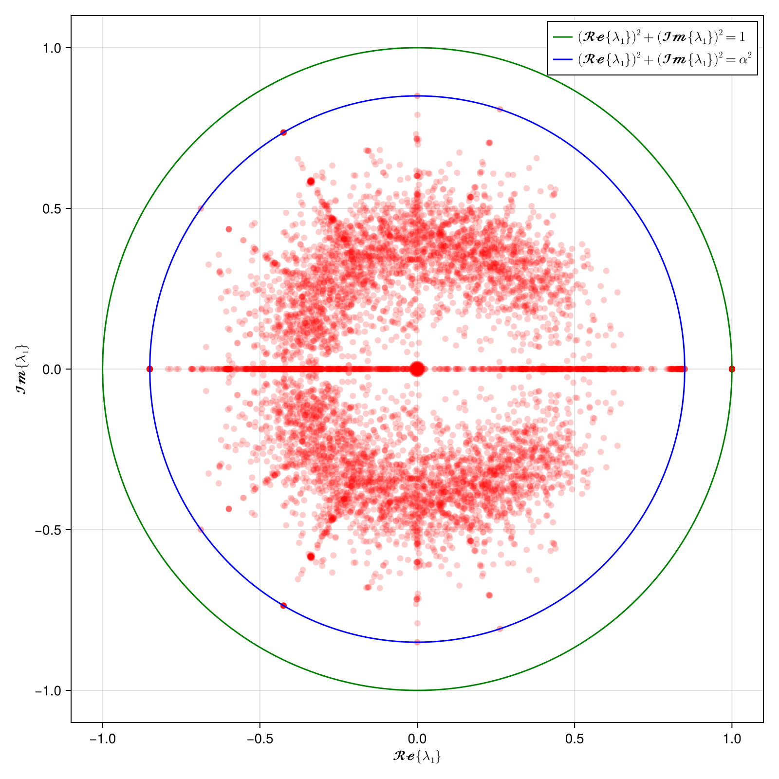
AS you can see there is a singular eigenvalue equal to 1. This is the principle eigenvalue (the perron frobenius eigenvalue) of our matrix coinciding with the unit circle drawn with real and imaginary part of the eigenvalues. The second largest eigenvalue is clearly bound by the parameter as discussed above. This big gap allows quick and accurate PageRank calculation.
Interesting to note protrusions of 'more stable' eigenvalues shown in star structure. There are some eigenvalues with higher magnitude that are at certain angles in the complex plane. Ermann et al,2015 while studying google matrix of empirical university network mentions these values:
These structures are very similar to those seen in the spectra of random orthostochastic matrices of small size N = 3, 4 shown in .... indicates that there are dominant triple and quadruple structures of nodes present in the University networks which are relatively weakly connected to other nodes.
Further, these values do not appear if we increase the value of significantly.
PageRank and Eigenvector centrality
The fact that the google matrix is a matrix that one obtains from the adjacency matrix, and PageRank is essentially the principle eigenvector (corresponding to largest eigenvalue), it intrigued me to identify how the eigenvector centrality is connected with PageRank of the network.
Ofcourse, PageRank works better for directed networks and is a more advanced version of the eigenvector centrality. Eigenvector centrality does not work for nodes with no incoming link. PageRank is able to takes care of those nodes too. So it should provide different results. But it could be an interesting exercise to compare these results.
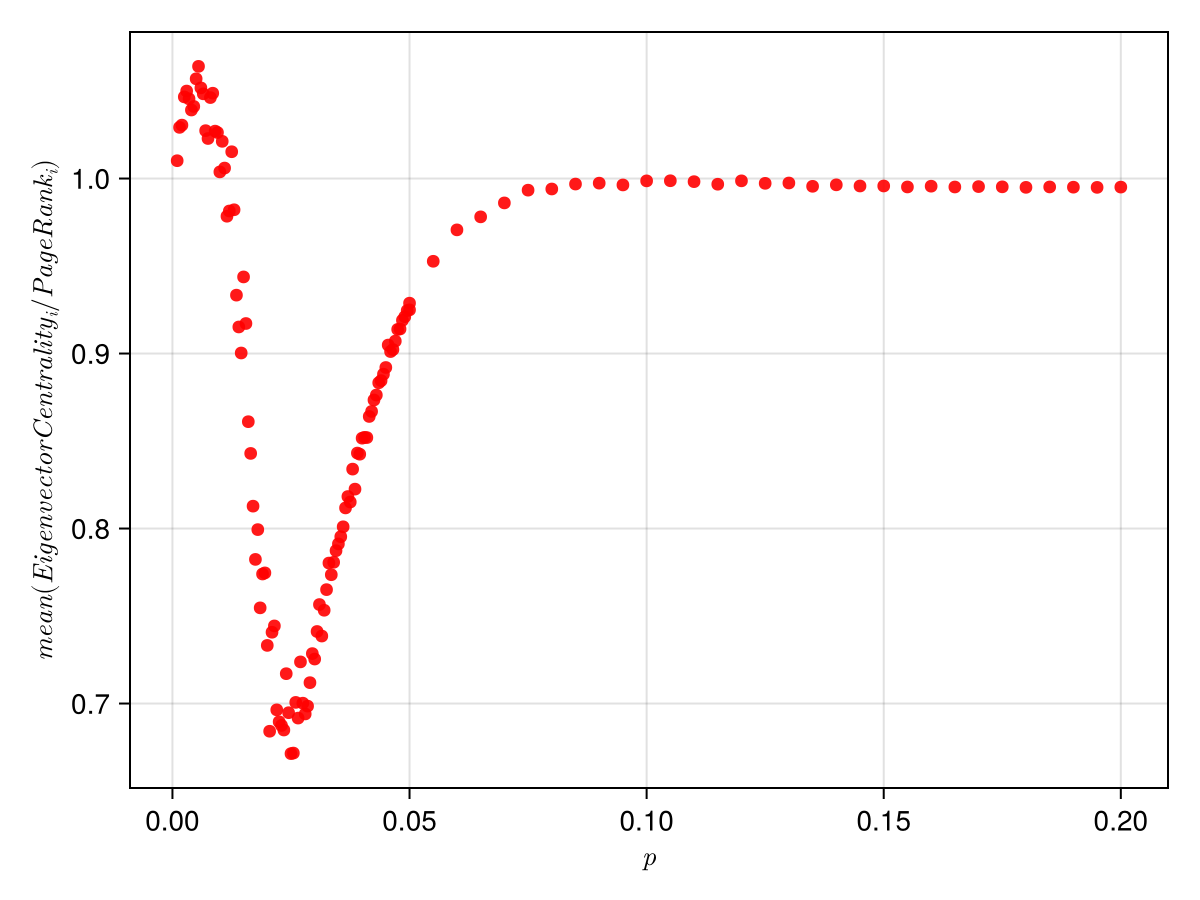
In the plot above you can see that both centrality measures converge to same results for higher value of connecting probability.
For lower values of probability, the ratio is higher than one, then once it dips below 1 it never gets back to 1. The reason why it is more than 1 is because in lower p values, the largest eigenvalue was often 1 and there is no unique eigenvector defined. And even if there is one, the eigenvector centrality is zero for many nodes which are not getting any incoming link, but page rank is non zero for such nodes. This forces the non zero values in the eigenvector centrality to be significantly bigger as the whole vector has to be normalised.
The dip in the ratio seemed to be because of the giant component phase transition that occurs in erdos reni random networks at . The dip is around 0.025, while the giant component transition occurs at 0.02. But this does not seem to be the case. To verify this I did the same for :
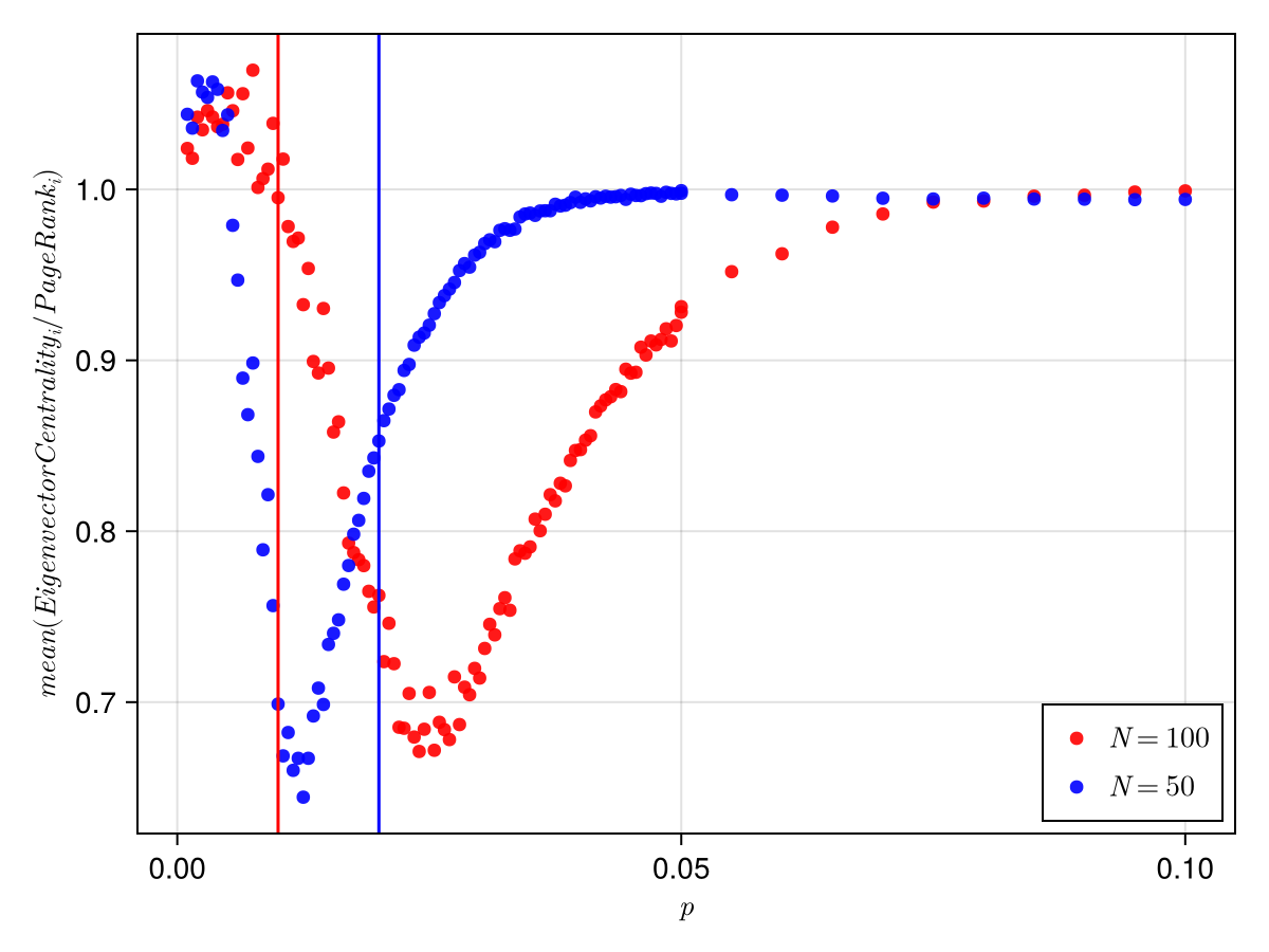
As we can clearly see, the transition takes place at a higher . If the transition was happening because of the giant component phase transition, then the minimum would have shifted to the left by increasing .
There is another transition seen in erdos renyi networks. Below the graph contains disconnected components and beyond this the graph becomes one connected entity. This threshold is for connectivity in the network. If we plot this as vertical lines with the ratio we get:
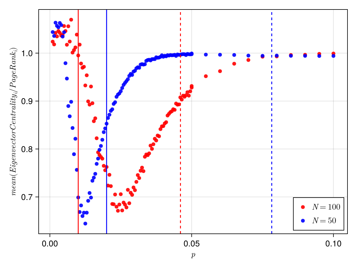
Although, the connectedness transition and the giant component transition does explain to a certain extent why the two centrality measures converge to same values. But the dip and its position is not exactly answered by the transitions.
It seems to me that a combinatorial effect of both transitions causes this dip and the dip's translation.
Since it is costlier to calculate PageRank compared to eigenvector centrality, it might be better to just use eigenvector centrality for more densely connected network. As we can see they on average give similar result.
This is it from me on this topic. But if I understand more things about this observation and I learn what is going on here, I will update this post or add another blog post.
Code for plots
#draw figure for eigenvalues with circles
prods=[]
L1s=[]
p=0.5
f=CairoMakie.Figure(size=(800,800))
ax=CairoMakie.Axis(f[1,1],xlabel=L"\mathcal{Re}\{\lambda_1\}",ylabel=L"\mathcal{Im}\{\lambda_1\}")
for itr in 1:500
    N=20
    p=1/N + 0.1
    A=zeros(Int8,N,N)
    for i in 1:N
        for j in 1:N
            if i!=j && rand()<p
                A[i,j]=1
            end
        end
    end
    G=google_matrix(DiGraph(A'),α=0.85,v = fill(1.0/N, N))
    vals,vecs=eigen(G)
    CairoMakie.scatter!(ax,real.(vals),imag.(vals),color=(:red,0.2))
end
xx=-1:0.001:1
a=0.85
xx1=-a:0.001:a
yy=sqrt.(1.0.- xx.*xx)
yy1=sqrt.(a*a .-xx1.*xx1)
CairoMakie.lines!(ax,xx,yy,color=:green,label=L"(\mathcal{Re}\{\lambda_1\})^2 + (\mathcal{Im}\{\lambda_1\})^2 = 1 ")
CairoMakie.lines!(ax,xx,-yy,color=:green)
CairoMakie.lines!(ax,xx1,yy1,color=:blue,label=L"(\mathcal{Re}\{\lambda_1\})^2 + (\mathcal{Im}\{\lambda_1\})^2 = (1-\alpha)^2 ")
CairoMakie.lines!(ax,xx1,-yy1,color=:blue)
axislegend(ax)
f

prods=[]
PRODS=[]
L1s=[]
p=0.5
sds1=[]
means1=[]
parr=[0.002,0.005,0.01,0.1,0.2,0.3,0.5,0.7,0.9]
parrlow=0.001:0.0005:0.05
parrhigh=0.05:0.005:0.1
parr=[]
x=vcat(parr,parrlow)
parr=vcat(x,parrhigh)
for p in parr
    f=CairoMakie.Figure()
    ax=CairoMakie.Axis(f[1,1])
    PRODS1=[]
    for itr in 1:500
        N=100
        A=zeros(Int8,N,N)
        for i in 1:N
            for j in 1:N
                if i!=j && rand()<p
                    A[i,j]=1
#                    A[j,i]=1
                end
            end
        end
        G=google_matrix(DiGraph(A'),α=0.85,v = fill(1.0/N, N))
        vals,vecs=eigen(G)
        evals,evecs=eigen(A)
        x1=abs.(real.(vecs[:,N]))
        x1=x1./sum(x1)
        x2=abs.(real.(evecs[:,N]))
        x2=x2./sum(x2)
        L1=maximum(real.(evals))
        append!(prods,(x2./x1)[1])
        append!(L1s,L1)
        push!(PRODS,x2./x1)
        push!(PRODS1,x2./x1)
    #    CairoMakie.scatter!(ax,real.(evals),imag.(evals),color=(:blue,0.2))
    #    println((x1./x2)[1],"\t",L1,"\t",var(x1./x2),"\t",L1*√2)
    end
    append!(means1,mean(mean.(PRODS1)))
    append!(sds1,sqrt(var(mean.(PRODS1))))
#    println(mean(prods),"\t",sqrt(var(prods)))
end
CairoMakie.scatter!(ax,parr,means1,color=(:red,0.2))
f

using SparseArrays, Graphs, LinearAlgebra

"""
    google_matrix(g::DiGraph; α=0.85, v::AbstractVector = nothing)

Construct the Google matrix G = α S + (1-α) v*1' for a directed graph g.

- S is the column-stochastic transition matrix built from the adjacency with dangling columns replaced by uniform 1/N.
- α is the damping factor (typical value 0.85).
- v is a personalization (teleportation) distribution (length N, nonnegative, sums to 1). If not provided, v = fill(1/N, N).

Returns a SparseMatrixCSC{Float64,Int}.
"""
function google_matrix(g::DiGraph; α=0.85, v::AbstractVector = nothing)
    N = nv(g)
    N == 0 && return spzeros(0,0)
    v === nothing && (v = fill(1.0/N, N))
    @assert length(v) == N && all(>=(0), v) && isapprox(sum(v), 1.0; atol=1e-12)

    # Build column-stochastic S from adjacency A with columns normalized by out-degree (dangling columns -> 1/N)
    rows = Int[]
    cols = Int[]
    vals = Float64[]
    outdeg = outdegree.(Ref(g), 1:N)

    # Fill columns by iterating over edges (u -> w means column u contributes to row w)
    for u in 1:N
        if outdeg[u] > 0
            w = 1.0 / outdeg[u]
            for wv in outneighbors(g, u)
                push!(rows, wv)
                push!(cols, u)
                push!(vals, w)
            end
        else
            # Dangling column: uniform distribution 1/N in column u
            for i in 1:N
                push!(rows, i)
                push!(cols, u)
                push!(vals, 1.0/N)
            end
        end
    end
    S = sparse(rows, cols, vals, N, N)

    # Google matrix: G = α S + (1-α) v*1'
    # Implement efficiently as sparse plus low-rank term
    oneT = fill(1.0, 1, N)          # 1' row vector
    G = α * S + (1-α) * (v * oneT)  # Dense low-rank update; result is dense unless α≈1
    return G
end
f=CairoMakie.Figure()
ax=CairoMakie.Axis(f[1,1],
    #xscale=log10,
    xlabel=L"p",ylabel=L"mean(EigenvectorCentrality_i/PageRank_i)")
#CairoMakie.errorbars!(ax,parr,means,sds,color=(:pink,0.7))
N=100
CairoMakie.scatter!(ax,parr,means,color=(:red,0.9),label=L"N=100")
CairoMakie.scatter!(ax,parr,means1,color=(:blue,0.9),label=L"N=50")

CairoMakie.vlines!(ax,1/N,color=:red)
CairoMakie.vlines!(ax,log(N)/N,color=:red,linestyle=:dash)

CairoMakie.vlines!(ax,1/50,color=:blue)
CairoMakie.vlines!(ax,log(50)/50,color=:blue,linestyle=:dash)

axislegend(ax,position=:rb)
#CairoMakie.save("/home/azafar/Desktop/GitHub/atiyabzafar.github.io/Blog/2025/images/ratio_50_500_100_500_transition.png",f)
f