A Physicist and a mathematician loves pattern and you can see the rare twinkle in their eyes (when the dread has not set in) when they find the patterns in unexpected places. And so it was the case recently with me when i found pi, the universal constant that arise from geometry of a circle in an unexpected place (Although purely co-incidentally)
Now pi has been a fascination for me for a long long time, ever since i started studying geometry in school and the fascination just grew exponentially. You can check out my last post on the blog which was my first love letter to pi, in which i talk about various ways to calculate including Monte Carlo method.
The beauty of it never ends too
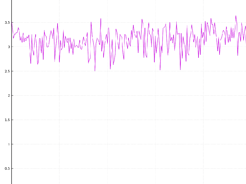
Graph showing the same
So, I have been working with non linear dynamical equation and solving a set of equations numerically using RK4 solver.(To those of you who don't know RK4 is a Runge Katta algorithm to solve Differential Equations), I had a complicated enough system of multiple equations and I ran my algorithm, as the program started giving me output , I saw numbers flashing by my screen. 3.25, 3.43, 2.91, ... and there I was sitting in the library giggling like a 3 year old as I witnessed \(\pi\) coming out as time it takes to reach the attractor(final state).
But as obvious once I changed the step size of my ode solver the final time changed. (Halving the step size took twice as much time thus tending to \(2\pi\).) But this post is not meant for this simulation. This post is to explore other such examples where pi creeps in. Most astonishing being the Mandelbrot Set.
Gaussian Integral
Gaussian Integral is the integral of Gaussian function : \(e^{-x^2}\)
\[\int _{-\infty }^{\infty }e^{-x^{2}}\,dx={\sqrt {\pi }}\]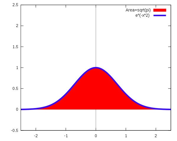
Source: Wikimedia
Now we can write a whole post about the applications and importance of gaussian function and normal distribution, applications of the function range from statistics to natural science. It's interesting how the ratio of circumference of a circle to the diameter appears in integral of a distribution function that on first glance has no connection to a circle. It's not difficult to show the relation of spherical symmetry and circle to this integral. Click below to see the derivation and connection:
\[ \left(\int _{-\infty }^{\infty }e^{-x^{2}}\,dx\right)^{2}=\int _{-\infty }^{\infty }e^{-x^{2}}\,dx\int _{-\infty }^{\infty }e^{-y^{2}}\,dy=\int _{-\infty }^{\infty }\int _{-\infty }^{\infty }e^{-(x^{2}+y^{2})}\,dx\,dy\]In polar co-ordinates, we can show \(r^2=x^2+y^2\) and \(dx dx= r dr d \theta\) , thus the integral can be solved as :
\[\begin{aligned} \left(\int _{-\infty }^{\infty }e^{-x^{2}}\,dx\right)^{2}&=\int _{0}^{2\pi }\int _{0}^{\infty }e^{-r^{2}}r\,dr\,d\theta \\\&=2\pi \int _{0}^{\infty }re^{-r^{2}}\,dr\\\&=2\pi \int _{-\infty }^{0}{\tfrac {1}{2}}e^{s}\,ds&&s=-r^{2}\\\&=\pi \int _{-\infty }^{0}e^{s}\,ds\\\&=\pi (e^{0}-e^{-\infty })\\\&=\pi ,\end{aligned}\]Thus taking square-root of both sides we get \(\sqrt\\pi\) . There's always a circle around.
\[/bg_collapse\]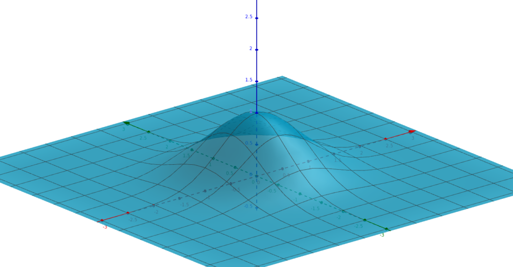
Surface plot of exp(-x*x-y*y)
π in Oscillations
You get π in any oscillation. When a mass bobs on a spring, or a pendulum swings back and forth, the position behaves just like one coordinate of a particle going around a circle in the phase space.
The catch starts with physicist's favorite assumption , As shown in this wired article titled : Everything—Yes, Everything—Is a Harmonic Oscillator
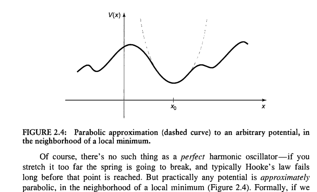
My favourite depiction of Harmonic Oscillator assumption from Griffiths: Introduction to Quantum Mechanics
If we boldly go there, we can assume any dynamical system to be locally harmonic around a minima and thus have a periodic circular motion and therefore have pi appearing in the expression for the Time period.
π as a matrix eigenvalue
This is a wild one : It can be shown that for a Tri-diagonal Matrix of the form :
\[M=m^2\left( \begin{array}{cccccc} -2 & 1 & 0 & \cdots & \cdots & 0 \ 1 & -2 & 1 & \cdots & \cdots & 0 \\ 0 & 1 & -2 & 1 & \cdots & 0 \\ \vdots & \cdots & \vdots & \vdots & \cdots & \vdots \\ 0 & \cdots & \cdots & 1 & -2 & 1 \\ 0 & \cdots & \cdots & 0 & 1 & -2 \\ \end{array} \right).\]The square root of absolute value of largest eigen value tends to value of pi as m tends to infinity. (Source at the end)
\[2m^2-2{m^2}\cos \left({\frac {k\pi }{n+1}}\right),\qquad k=1,\ldots ,n\]If you take large m approximation in the expression above you can show the result analytically tending to \(\pi\)
For example I did a quick numerical calculation by using R and found for m=100 largest eigen value is : -9.674354 which gives me approximate value of pi to be 3.110362.
<table class="wp-block-table is-style-stripes"><tbody><tr><td>m</td><td>Value of Square root of |largest Eigen Value|</td></tr><tr><td>10</td><td>2.846297</td></tr><tr><td>100</td><td>3.110362</td></tr><tr><td>1000</td><td>3.1384</td></tr><tr><td>5000<br></td><td>3.140964</td></tr></tbody></table>
n=100
m <- diag(-2\*n\*n, n)
m\[abs(row(m) - col(m)) == 1\] <- n\*n
ev<-eigen(m)$values
p2=max(ev)
p=sqrt(abs(p2))
π in Mathematics' most beautiful function (IMO)
The Riemann zeta function ζ(s), is a function of a complex variable s :
\[\zeta (s)=\sum_{n=1}^{\infty}{\frac {1}{n^{s}}}\]With applications from Statistical Physics, to number theory Riemann Zeta function holds in itself some incredibly astonishing properties (Think of s=-1 case), if we consider s=2 the function converges to :
\[\zeta (2)=1+{\frac {1}{2^{2}}}+{\frac {1}{3^{2}}}+\cdots ={\frac {\pi ^{2}}{6}}\approx 1.64493406684822643647; \]This problem is famous Basel Problem that was solved by Euler himself back in late 1700s. Here is a very beautiful geometric proof explaining where and how the circle comes in and donates the pi in the expression.
π in the Mandelbrot set
This is the most interesting bit i could find. It's astonishingly brilliant!.
So for those who don't know Mandelbrot set arrives from the complex logistic equation, \(z_{n+1}=z_{n}^{2}+c\). We start from \(z_0=0\) and reiterate the expression , we map this for various values of complex number c.
Thus, a complex number \(c\) is a member of the Mandelbrot set if, when starting with \(z_0 = 0\) and applying the iteration repeatedly, the absolute value of \(z_n\) remains bounded for all \(n>0\).
For example, for \(c_=1\), the sequence is 0, 1, 2, 5, 26, ..., which tends to infinity, so 1 is not an element of the Mandelbrot set. On the other hand, for c =−1, the sequence is 0, −1, 0, −1, 0, ..., which is bounded, so −1 does belong to the set. (Source:http://math.bu.edu/DYSYS/explorer/def.html)

This is the Mandelbrot Set(Black)
Okay so I hope you are still here with me, the beautiful self repeating pattern that we have just got again has immense interesting qualities which we will be going after in another post later on.
What I am going to verify here has blown my mind and i hope you find it interesting too. If we look at a boundary point of the Mandelbrot Set, say c=0.25 or 1/4, we can show that it converges to 1/2.
\[\begin{aligned} z_1 &= 0*0+0.25=1/4 \\ z_2 &= (1/4)*(1/4) + 0.25 =5/16 \\ ... & so \quad on \end{aligned}\]Now since we are at the boundary of the set, if I add a small number to c, (i.e \(c \to c + \delta\) where \(\delta\) is a small number), the value should diverge to infinity.
Now let's calculate the Rate of Escape, something like escape velocity in complex space, defining the rate as the number of steps the equation takes so that \(z_n>2\).
So Rate of Escape : \(N(\delta)=\) No. of iterations it takes until \(z_n>2.0.\)
For example : if \(\delta=0.1\) the iterations looks something like this
<table class="wp-block-table has-fixed-layout"><tbody><tr><td>\(Z_n\)</td><td>0.26</td><td>0.35</td><td>0.4725</td><td>0.573256</td><td>0.678623</td><td>0.810529</td><td>1.006957</td><td>1.363962</td><td>2.210393</td></tr><tr><td>\(z_{n+1}\)</td><td>0.35</td><td>0.4725</td><td>0.573256</td><td>0.678623</td><td>0.810529</td><td>1.006957</td><td>1.363962</td><td>2.210393</td><td>-</td></tr></tbody></table>
So here it took 8 steps, now we multiply this number by square root of the original deviation and get 2.5298..., Hmmm, not really interesting yet
Here is a simple C program I wrote to find out the same quantity \(P=N(\delta)\sqrt{\delta}\)
#include <stdio.h>
#include <math.h>
int main()
{
	double z0=0,z1,c=0.25,d=0.1;
	c=c+d;
	do
	{
	z0=0;
	c=0.25;
	c=c+d;
		int p=0;
		do
		{
		z1=z0\*z0+c;
		z0=z1;
		p++;
		}while(z1<2.0);
		printf("%d\t%1.12lf\t%1.14lf\n",p,d,p\*sqrt(d));
	d=d\*0.1;
	}while(d>1e-11);
	return 0;
}
Compiled below is the result for various values of \(\delta\)
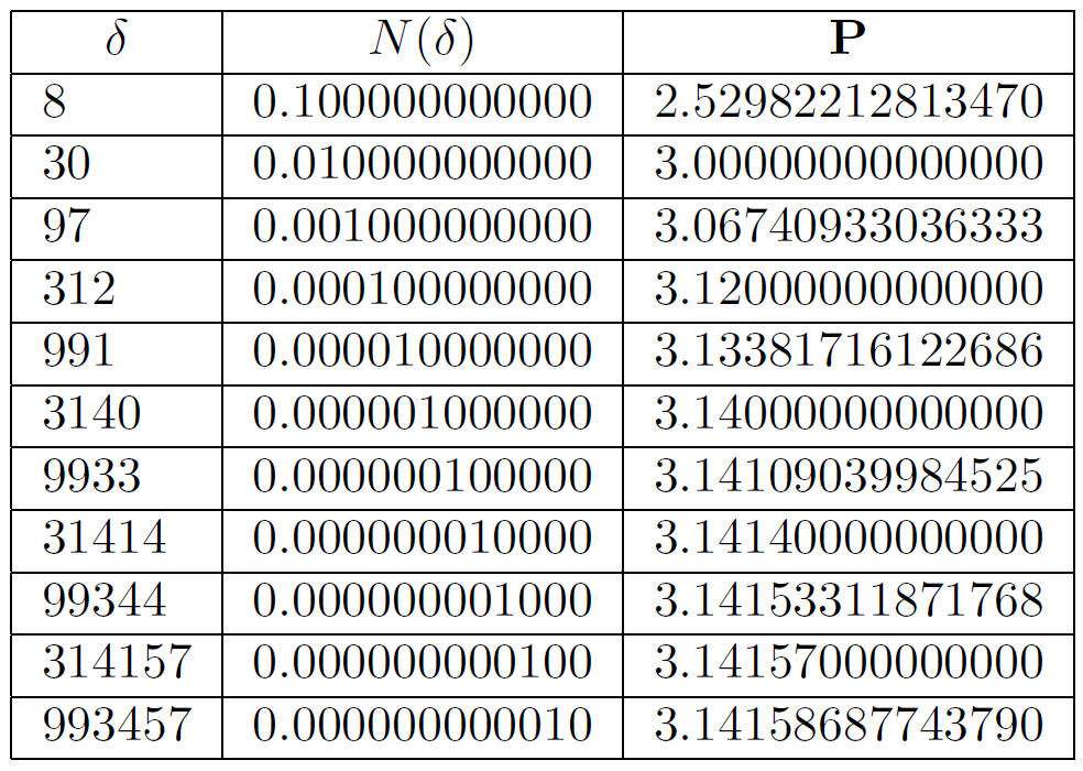
As \(\delta\) goes down the value of P goes to Pi!
This astonishing result was first shown in 1991. It lead to even further research in the field of Julia and Mandelbrot Set.
We can go on about the beauty of this number, so i'll save some more for my next love letter. Untill then stay Curious folks :).
SOURCE: main source of inspiration this blog post was based on : https://math.stackexchange.com/questions/689315/interesting-and-unexpected-applications-of-pi
title: "Surprising Places where Pi pops up |Celebrating Pi Day:Love Letters to Pi" date: "2020-03-14" categories:
"mathematics"
"physics"
tags:
"mathematics"
"pi-day"
coverImage: "PiNeverEnds2-1.png"